Beyond the Bell Curve: A Beginner’s Visual Guide to Distributions in Quantitative Trading

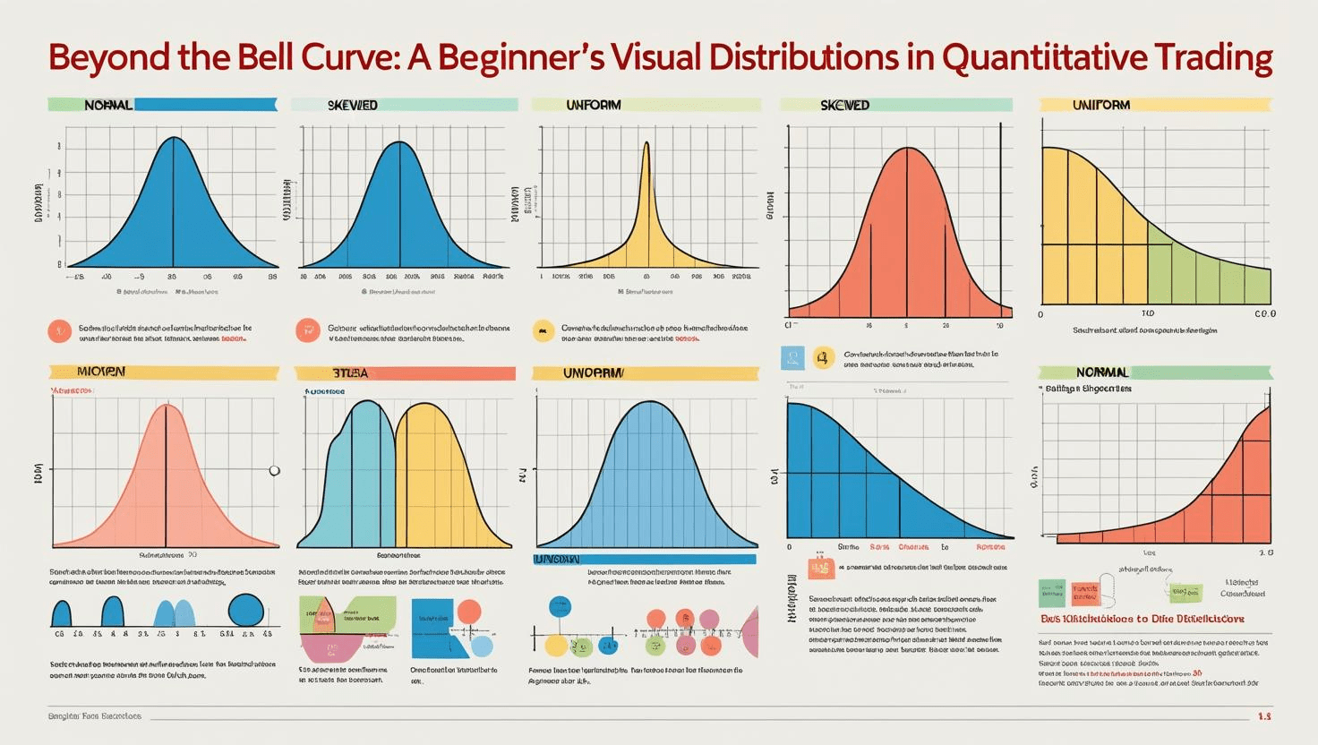
What are Distributions and Why Do They Matter?

In quantitative trading, we often deal with vast amounts of data: stock prices, returns, volumes, and more. A **distribution** is simply a way to describe how this data is spread out or how often different values occur. Think of it as a fingerprint for your data. Understanding these patterns is crucial because it helps traders:

**Quantify Risk:** How likely are extreme price movements?
**Develop Strategies:** What’s the probability of a trade being profitable?
**Make Informed Decisions:** Are market movements normal, or are there hidden risks?

Let’s explore some fundamental distributions that every aspiring quant trader should know.

1. The Normal Distribution (The “Bell Curve”)

Concept: The Symmetrical Average

The Normal Distribution, also known as the Gaussian distribution, is one of the most common probability distributions. It’s symmetrical, with data clustering around the mean (average), and tapering off evenly on both sides, forming a “bell” shape.

Relevance in Trading: A Starting Point (But Often Imperfect)

Historically, asset returns were often assumed to follow a normal distribution for simplicity in financial models. While easy to work with, real-world financial returns rarely fit this perfect bell curve, especially when considering extreme events.

2. The Log-Normal Distribution

Concept: Prices Can’t Go Below Zero

Unlike returns, asset *prices* cannot be negative. The Log-Normal distribution is used when the logarithm of a variable is normally distributed. This makes it naturally skewed to the right, reflecting that prices can increase indefinitely but only fall to zero.

Relevance in Trading: Modeling Asset Prices

This distribution is often a more realistic model for asset prices over time. It’s fundamental in option pricing models like Black-Scholes, where the underlying asset’s price is assumed to follow a log-normal path.

3. Student’s t-Distribution (“Fat Tails”)

Concept: More Extreme Events

The Student’s t-distribution resembles the normal distribution but has “fatter tails.” This means it assigns a higher probability to extreme outcomes (both positive and negative) compared to the normal distribution.

Relevance in Trading: Real-World Financial Returns

This is crucial for financial modeling because real-world market returns often exhibit “fat tails” – large price movements occur more frequently than a perfectly normal distribution would predict. Using the t-distribution helps quants better account for “tail risk” or black swan events.

4. Bernoulli & Binomial Distributions (Win/Loss Probabilities)

Bernoulli: Single Trade Outcome

The Bernoulli distribution models a single experiment with two possible outcomes: success (e.g., a winning trade) or failure (a losing trade). Each outcome has a fixed probability.

Binomial: Series of Trades

The Binomial distribution describes the number of successes in a fixed number of independent Bernoulli trials. For example, how many winning trades you might have in a series of 100 trades, given your historical win rate.

5. Uniform Distribution

Concept: Equal Probability for All Outcomes

In a Uniform distribution, every value within a given range has an equal probability of occurring. It’s a “flat” distribution, indicating no particular bias towards any specific value.

Relevance in Trading: Simulations & Randomness

While raw market data rarely follows a uniform distribution, it’s very useful in quantitative trading for simulations like Monte Carlo methods. You might generate random numbers from a uniform distribution to simulate various market scenarios or test strategies under random conditions.

Why These Distributions Matter to Quants

**Risk Management:** Knowing the distribution of returns allows quants to calculate Value-at-Risk (VaR) or Expected Shortfall (ES), helping quantify potential losses with specific probabilities.
**Strategy Backtesting & Optimization:** Distributions are used to understand the statistical edge of a trading strategy and to optimize parameters like stop-loss and take-profit levels.
**Derivative Pricing:** Complex financial instruments like options are priced based on assumptions about how the underlying asset’s price will move (often using log-normal distributions).
**Market Simulation:** Quants use distributions to generate synthetic market data for stress testing strategies or exploring hypothetical scenarios through Monte Carlo simulations.
**Identifying Anomalies:** Deviations from expected distributions can signal unusual market behavior, potential arbitrage opportunities, or emerging risks.

Algo Trading Byte