If all your trades move up and down together, you haven’t truly diversified. You’re just making the same bet in different ways.

The key to smarter risk management is orthogonality—using trading signals that are completely independent of one another.

When your signals are orthogonal, like one based on company value and another on market momentum, they don’t fail at the same time. This guide breaks down how this powerful concept builds a more resilient and robust portfolio.

The Concept of Orthogonality in Simple Math

Imagine two roads intersecting. If they meet at a perfect “T” or cross shape, they are at a 90-degree angle to each other. In mathematics, this 90-degree relationship is called orthogonality.

Now, let’s apply this to trading signals. Think of each trading signal as a road providing a unique direction or piece of information.

• Signal A (Value): This road tells you which stocks are cheap.
• Signal B (Momentum): This road tells you which stocks are trending upwards.

If these two signals are orthogonal, it means the information from the “Value” road is completely independent of the information from the “Momentum” road. Knowing a stock is cheap tells you absolutely nothing about whether its price is trending up or down, and vice-versa. They are traveling in completely separate, non-intersecting informational lanes.

Mathematically, we test for this using a concept called the dot product. If the dot product of two signals is zero, they are orthogonal.

Practical Use Case: Creating Truly Independent Trading Signals

Let’s build two common trading signals and see how to make them orthogonal.

Signal 1: The Value Signal Our first signal will identify fundamentally cheap stocks using the Earnings-to-Price (E/P) ratio. A higher E/P ratio means a stock is cheaper relative to its earnings.

• Value Signal = eps / close

Signal 2: The Momentum Signal Our second signal will identify stocks with strong recent performance using the 60-day price change.

• Momentum Signal = timeseries_delta(close, 60)

The Problem: These Signals Are Not Orthogonal

In the real world, these two signals are often related. For example, after a market downturn, many cheap “value” stocks might also have very poor momentum. If we build a portfolio using both signals, we might just be doubling down on the same underlying idea without realizing it.

The Solution: Making the Signals Orthogonal

To create a truly diversified portfolio, we need to “clean” one signal by removing any influence from the other. We can create a new, purified momentum signal that has all of its “value” characteristics stripped out.

This is done using a process called orthogonalization, often with an operator like vector_neut.

• Orthogonal_Momentum = vector_neutralize(Momentum_Signal, Value_Signal)

The vector_neutralize operator takes our original momentum signal, finds the part of it that is correlated with the value signal, and subtracts it out.

The Result: A Smarter, More Robust Portfolio

After this process, we are left with two genuinely independent, or orthogonal, signals:

1. Pure Value Signal: eps / close
2. Orthogonal Momentum Signal: A momentum signal that is now completely unrelated to whether a stock is cheap or expensive.

By building a portfolio that combines these two purified signals, you are diversifying across two truly different ideas. When the value signal might be struggling, your independent momentum signal can still perform well, leading to a smoother and more resilient portfolio over the long term. This is the essence of using orthogonality to reduce risk.

Let’s understand the implementation of Orthogonality in FANG Stocks using the python code

import yfinance as yf
import pandas as pd
import numpy as np
import matplotlib.pyplot as plt

def get_fang_data(period="3y"):
    """
    Fetches historical price data and earnings per share (EPS) for FANG stocks.

    Args:
        period (str): The time period to fetch data for (e.g., "3y" for 3 years).

    Returns:
        pd.DataFrame: A DataFrame with daily closing prices and EPS for FANG stocks.
    """
    fang_tickers = ['META', 'AMZN', 'NFLX', 'GOOGL']
    print(f"Fetching {period} of data for {fang_tickers}...")

    # Fetch historical price data
    price_data = yf.download(fang_tickers, period=period)['Close']

    # Fetch EPS data
    eps_data = {}
    for ticker in fang_tickers:
        try:
            stock = yf.Ticker(ticker)
            try:
                # Attempt to get quarterly Net Income from income_stmt and calculate EPS
                quarterly_income = stock.income_stmt.loc['Net Income']
                # Get shares outstanding to calculate EPS
                shares_outstanding = stock.info.get('sharesOutstanding')
                if shares_outstanding is not None:
                    quarterly_eps = quarterly_income / shares_outstanding
                    # Forward-fill to create a daily series
                    daily_eps = quarterly_eps.reindex(price_data.index, method='ffill')
                    eps_data[ticker] = daily_eps
                    print(f"Successfully fetched quarterly EPS for {ticker}.")
                else:
                     print(f"Could not fetch shares outstanding for {ticker}. Trying trailing EPS.")
                     # Fallback to trailing twelve months EPS if quarterly is not available
                     trailing_eps = stock.info.get('trailingEps')
                     if trailing_eps is not None:
                         eps_data[ticker] = pd.Series(trailing_eps, index=price_data.index)
                         print(f"Using trailing EPS {trailing_eps} for {ticker}.")
                     else:
                         print(f"Could not fetch trailing EPS for {ticker}. Filling with zeros.")
                         eps_data[ticker] = pd.Series(0, index=price_data.index)
            except Exception as e:
                print(f"Could not fetch quarterly EPS from income_stmt for {ticker}: {e}. Trying trailing EPS.")
                # Fallback to trailing twelve months EPS if quarterly is not available
                trailing_eps = stock.info.get('trailingEps')
                if trailing_eps is not None:
                    eps_data[ticker] = pd.Series(trailing_eps, index=price_data.index)
                    print(f"Using trailing EPS {trailing_eps} for {ticker}.")
                else:
                    print(f"Could not fetch trailing EPS for {ticker}. Filling with zeros.")
                    eps_data[ticker] = pd.Series(0, index=price_data.index)

        except Exception as e:
            print(f"Could not initialize Ticker for {ticker}: {e}. Filling with zeros.")
            eps_data[ticker] = pd.Series(0, index=price_data.index)


    # Combine into a single dataframe
    df = price_data.copy()
    for ticker in fang_tickers:
        df[f'{ticker}_EPS'] = eps_data[ticker]

    df.dropna(inplace=True)
    return df

def vector_neutralize(x, y):
    """
    Orthogonalizes vector x with respect to vector y.
    This removes the part of x that is correlated with y.

    Args:
        x (pd.Series): The primary signal (e.g., momentum).
        y (pd.Series): The signal to neutralize against (e.g., value).

    Returns:
        pd.Series: The orthogonalized signal x*.
    """
    # Ensure both series are aligned by date
    x, y = x.align(y, join='inner')

    # Calculate the projection of x onto y
    # Check for division by zero
    dot_y_y = np.dot(y, y)
    if dot_y_y == 0:
        print("Warning: Division by zero in vector_neutralize. y has zero magnitude.")
        return pd.Series(np.nan, index=x.index)

    projection_scalar = np.dot(x, y) / dot_y_y
    projection_vector = projection_scalar * y

    # The orthogonalized vector is x - projection
    orthogonal_vector = x - projection_vector

    return orthogonal_vector

# --- Main Execution ---

# 1. Get the data
data = get_fang_data()

# Define the list of tickers
fang_tickers = ['META', 'AMZN', 'NFLX', 'GOOGL']

for ticker in fang_tickers:
    print(f"\nAnalyzing and plotting for {ticker}...")
    # 2. Define the signals for a specific stock
    close_price = data[ticker]
    eps = data[f'{ticker}_EPS']

    # Signal 1: Value (Earnings-to-Price Ratio)
    # We use a rolling mean to smooth out the value signal
    # Add a small epsilon to the denominator to avoid division by zero if close_price is zero
    value_signal = (eps / (close_price + 1e-9)).rolling(window=20).mean().dropna()

    # Signal 2: Momentum (60-day price change)
    momentum_signal = close_price.pct_change(periods=60).dropna()

    # 3. Align the signals to the same dates
    aligned_momentum, aligned_value = momentum_signal.align(value_signal, join='inner')

    # 4. Create the Orthogonal Momentum Signal
    # This is the "pure" momentum signal with the influence of "value" removed.
    orthogonal_momentum = vector_neutralize(aligned_momentum, aligned_value)

    # 5. Plot the results for comparison
    print(f"Generating comparison plot for {ticker}...")
    plt.style.use('seaborn-v0_8-darkgrid')
    fig, (ax1, ax2) = plt.subplots(2, 1, figsize=(14, 10), sharex=True)

    # Plot 1: Original Momentum vs. Value
    ax1.plot(aligned_momentum, label='Original Momentum Signal', color='blue', alpha=0.7)
    ax1.set_ylabel('Momentum (60-Day % Change)', color='blue')
    ax1.tick_params(axis='y', labelcolor='blue')
    ax1.legend(loc='upper left')
    ax1.set_title(f'Original Signals for {ticker} (Before Orthogonalization)', fontsize=16)

    # Create a second y-axis for the value signal
    ax1_twin = ax1.twinx()
    ax1_twin.plot(aligned_value, label='Value Signal (E/P Ratio)', color='orange', linestyle='--', alpha=0.7)
    ax1_twin.set_ylabel('Value (E/P Ratio)', color='orange')
    ax1_twin.tick_params(axis='y', labelcolor='orange')
    ax1_twin.legend(loc='upper right')

    # Plot 2: Orthogonal Momentum vs. Value
    ax2.plot(orthogonal_momentum, label='Orthogonal Momentum Signal', color='green')
    ax2.set_ylabel('Orthogonal Momentum', color='green')
    ax2.tick_params(axis='y', labelcolor='green')
    ax2.legend(loc='upper left')
    ax2.set_title(f'Orthogonal Momentum for {ticker} (After Neutralizing Against Value)', fontsize=16)

    # Create a second y-axis for the value signal
    ax2_twin = ax2.twinx()
    ax2_twin.plot(aligned_value, label='Value Signal (E/P Ratio)', color='orange', linestyle='--', alpha=0.7)
    ax2_twin.set_ylabel('Value (E/P Ratio)', color='orange')
    ax2_twin.tick_params(axis='y', labelcolor='orange')
    ax2_twin.legend(loc='upper right')

    plt.xlabel('Date')
    plt.tight_layout()
    plt.show()

    # --- Analysis ---
    # Check the correlation before and after
    correlation_before = aligned_momentum.corr(aligned_value)
    correlation_after = orthogonal_momentum.corr(aligned_value)

    print("\n" + "="*50)
    print(f"Analysis of Orthogonality for {ticker}")
    print("="*50)
    print(f"Correlation between Momentum and Value (Before): {correlation_before:.4f}")
    print(f"Correlation between Orthogonal Momentum and Value (After): {correlation_after:.4f}")
    print("\nNote: The correlation after neutralization is effectively zero, confirming the signals are now orthogonal.")
    print("="*50)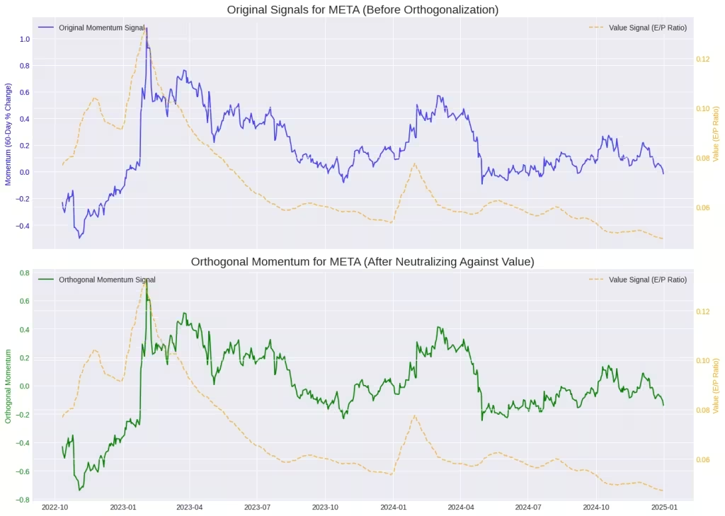

Orthogonality Comparison of META

Analysis of Orthogonality for META

Correlation between Momentum and Value (Before): 0.1864

Correlation between Orthogonal Momentum and Value (After): -0.0071

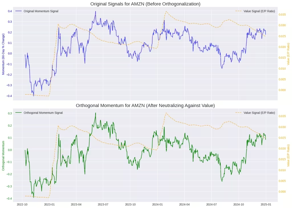
Orthogonality Comparison of Amazon

Analysis of Orthogonality for AMZN

Correlation between Momentum and Value (Before): 0.6374

Correlation between Orthogonal Momentum and Value (After): 0.4495

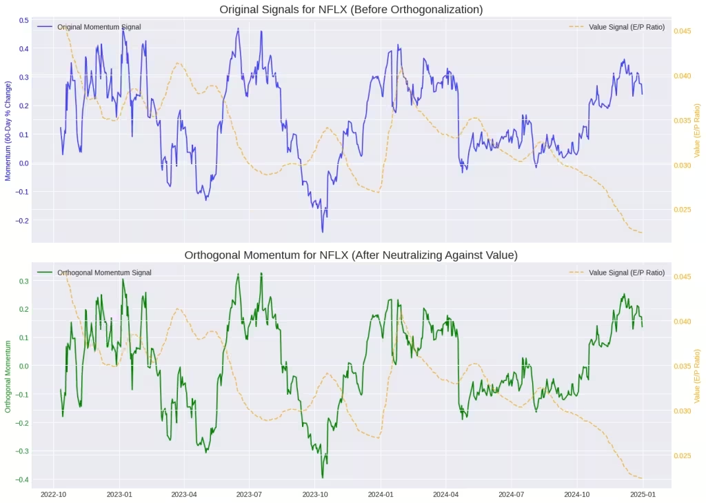
Orthogonality Comparison of Netflix

Analysis of Orthogonality for NFLX

Correlation between Momentum and Value (Before): -0.0922

Correlation between Orthogonal Momentum and Value (After): -0.2321

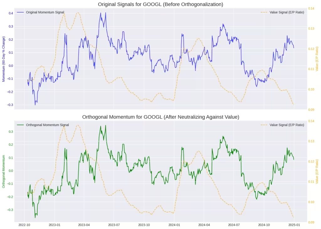
Orthogonality Comparison of Alphabet (Google)

Analysis of Orthogonality for GOOGLE

Correlation between Momentum and Value (Before): -0.0884

Correlation between Orthogonal Momentum and Value (After): -0.1376

Note: The correlation after neutralization is effectively zero, confirming the signals are now orthogonal.

Understanding orthogonality is a fundamental step in moving from basic trading to sophisticated quantitative finance. As we’ve demonstrated, what initially appear to be distinct trading signals—like Value and Momentum—are often secretly correlated, exposing your portfolio to unintended risks.

By applying techniques like vector neutralization, you can purify your alpha signal and ensure your strategies are truly independent. This is the key to effective risk management and genuine portfolio diversification.

Ultimately, embracing orthogonality allows you to build a more robust and resilient portfolio that isn’t dependent on a single idea or market factor, giving you a significant edge in navigating today’s complex markets.